Write-up - Hack of Trades

SQL RANK, DENSE_RANK, ROW_NUMBER

SQL (Structured Query Language) is a very powerful tool to interact with databases as we all know.

Some more advanced functions, such as window functions in particular, are even more powerful! A window function, as the name may suggest, enables you to compute a row-level assignment based on a defined range or “window”. You can Google it if you’re still lost…

I want to primarily focus on 3 window functions in this write-up that are often [mistakenly] used interchangeably. It is very important to understand what differentiates RANK vs DENSE_RANK vs ROW_NUMBER, and when to use which one.

RANK

RANK assigns a sequential number to a record based on the partition and order by operators. For example, if we use RANK based on Price, this will rank each row based Price. In doing so, if multiple records share the same Price, they will share the same rank. The immediate next row with a different Price will have a different rank, however it will be incremented by the number of additional rows the prior rank had.

DENSE_RANK

DENSE_RANK works similar to the RANK function, in that it assigns a sequential number to a record based on the partition and order by operators. Where it differs is on the immediate row following a set of records that share the same rank. The DENSE_RANK window function will assign the very next sequential number of the preceding rank, unlike RANK. As a result, there are no gaps when using DENSE_RANK as opposed to RANK.

ROW_NUMBER

ROW_NUMBER brings something different and potentially more useful to the table. This assigns a sequential number (based on price for example) to each record, however no 2 records share the same row number. For example, if 2 or more records share the same price, they will still have a sequential rank (such as 1, 2, 3) instead of (1, 1, 1) if we had used RANK or DENSE_RANK instead.

Let’s suppose we have a dataset consisting of customer_id, item_id and price, and we’ve applied all 3 window functions as:

row_number() over (order by price)

rank() over (order by price)

dense_rank() over (order by price)

Here is the output we’d expect for each.

Customer_ID	Item_ID	Price	ROW_NUMBER	RANK	DENSE_RANK
1	228	200	1	1	1
1	255	200	2	1	1
1	212	200	3	1	1
2	900	500	4	4	2

Each of these 3 window functions are powerful and useful based on different scenarios. It’s important to understand when and how to use which one for proper results.

Category: SQL and Databases, Write-up | LEAVE A COMMENT

May 31

Full Outer Join in MySQL

If you’re familiar with databases and come from the Microsoft SQL Server world, you must love the ability to perform full outer joins when putting a dataset together.

Conversely, if you’re from the MySQL world, you must have no idea what I’m talking about since you cannot use full joins in MySQL.

Some Context

Let’s first understand the benefits of a full outer join to see why this would be valuable. Feel free to look at the video below to grasp an understanding of the intended output: Full Outer Join: SQL Tutorial with Example

How to Emulate a Full Outer Join

Now, you may be interested and want to replicate the full outer join in MySQL, but since it doesn’t offer support for this type of join, you will need to develop a workaround yourself.

Luckily, here is a straight forward approach to accomplishing this, using a combination of a left join, right join and union.

SELECT A.VALUE_A, B.VALUE_B
FROM A
LEFT JOIN B
ON A.VALUE_A= B.VALUE_B
UNION
SELECT A.VALUE_A, B.VALUE_B
FROM A
RIGHT JOIN B
ON A.VALUE_A= B.VALUE_B
;

The way this approach works, obviously, is it first performs a left or right join as a dataset, and then its counterpart (right or left join, respectively) as another dataset using the same query. This will give us “everything on the first table, even if the second table doesn’t have matching records” and also “everything on the second table, even if the first table doesn’t have matching records” as a second dataset. Then, by performing a union all, we stack these 2 datasets together and effectively combine them into one comprehensive dataset to give us “everything on the first and second table, regardless of whether or not they have matching values on their counterpart table”.

From an efficiency standpoint, yes, you are in fact querying twice as opposed to once which may not be ideal, however for the right use-case, this may be the right solution.

It’s really that simple!

Category: SQL and Databases, Write-up | LEAVE A COMMENT

April 30

Correctly Storing DB Credentials In PHP

There’s a way to do things, and then there’s a right way to do things. If you’ve been accustomed to storing your database login credentials inside or adjacent to your public-facing web application, you may benefit from this quick read.

In this write-up, I will show you the recommended approach to take to securely store and access your database credentials when working with PHP.

The Config File

First thing is first: in this example, I am using my shared hosting plan, and I assume you are too. What this means is you will be storing your web files somewhere under the public_html directory, which makes it publicly accessible. Our goal is to make a “private” folder outside of public_html that will be inaccessibly publicly, but accessible by our application residing in “public_html”.

Inside the private directory, we will create a file called config.ini that will store these credentials.

Enter your database credentials in this config.ini file as follows (obviously replacing the values in quotations with your own values).

config:ini

[database]
servername = “localhost”
username = “test_user”
password = “test_p4ssw0rd!”
dbname = “test_db”

Integration

Now, we can work on our php application under the public_html directory and point to the config file to parse the database credentials. Alternatively, you can call this in a separate file and then include the separate file in your main php application file, but for this short example we’ll just call it from the app directly. For more information on the parse_ini_file function, you can refer to the php documentation here

app.php

$config = parse_ini_file(‘../private/config.ini’);

In the same file, we can use PDO and reference the elements of $config to build a connection string and query our database.

try{
$_DB = new PDO(“mysql:host={$config[‘servername’]};dbname={$config[‘dbname’]}”, “{$config[‘username’]}”, “{$config[‘password’]}”);
$getIDs = $_DB->prepare(“Select * from employee_billing”);
$getIDs->execute();
$getEmpIDs = $getIDs->fetchAll();
foreach ($getEmpIDs as $emp){
echo “{$emp[’employee_id’]}
“;
}
}
catch (PDOException $e) {
die(“Error – connection failed. Please check your credentials or contact your administrator.”);
}

And this is all it takes to get your data to appear!

If you followed along, we just stood up a php application that uses a private, secure config file to supply its database credentials for connectivity.

Category: Web Development, Write-up | LEAVE A COMMENT

October 31

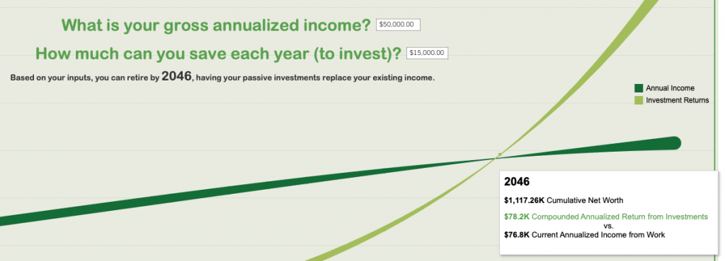
I built a dashboard to calculate when you can retire

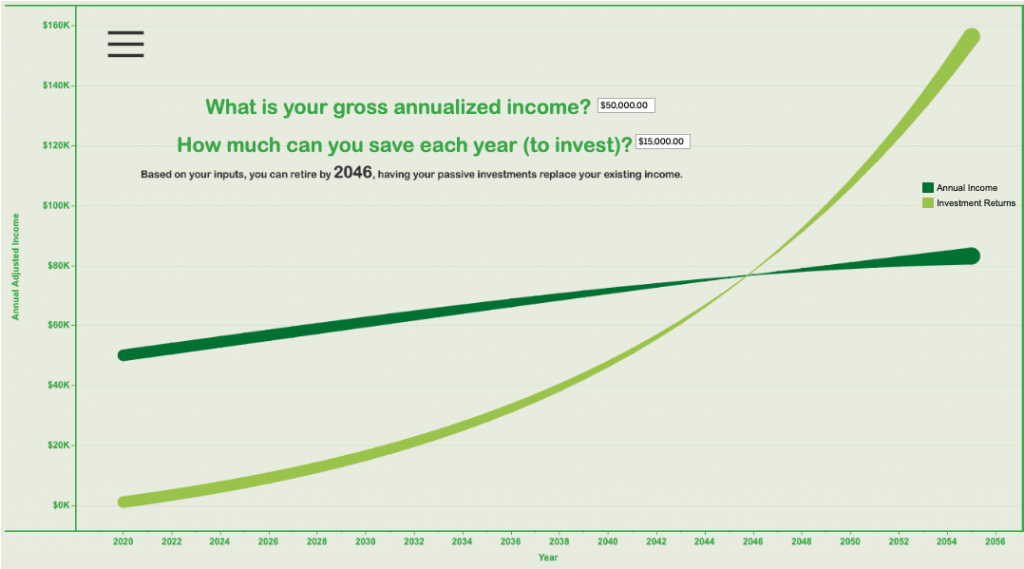
Using the awesome Tableau application once again, I was able to create an interactive visualization depicting the point in time an individual can expect to effectively converge or replace their active income with their passive investment income (generated from compounded earnings and investments).

One of the things I’m particularly proud of, is that this dashboard uses no data sources whatsoever. Everything is self contained in the workbook, which is simply an increasing sequence of “years” from 2020 upwards, and several calculated fields.

My goal was to keep this the best of all worlds between: simple, interactive and informative.

Users of this dashboards likely have varying levels of income and varying spending habits, so at the very least this dashboard should require 2 inputs: Gross Income and Annual Savings, to better personalize results.

The output in terms of the visualization should be, in its simplest form, 2 lines that intersect: Gross Annual Income and Change in Net Worth(synonymous to earnings from passive income/growth). What makes this challenging is that in a perfect world, neither the gross annual income – nor the passive income that is compounding will be stagnant throughout time. Both tend to trend upwards due to income raises and accumulated investments, respectively, over time. In short, the following is how the two output lines were generated.

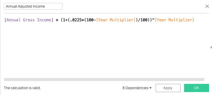
Annual Adjusted Income

This is the income generated from work. It will take the input, Annual Gross Income, and apply a raise of 2.25% compounded annually. There is also a somewhat arbitrary inverse of “Year Multiplier” I factored in, intended to reduce or taper-off that 2.25% raise over time as income from wages tends to slope downward late in careers (i.e. finding a new job as you approach retirement years).

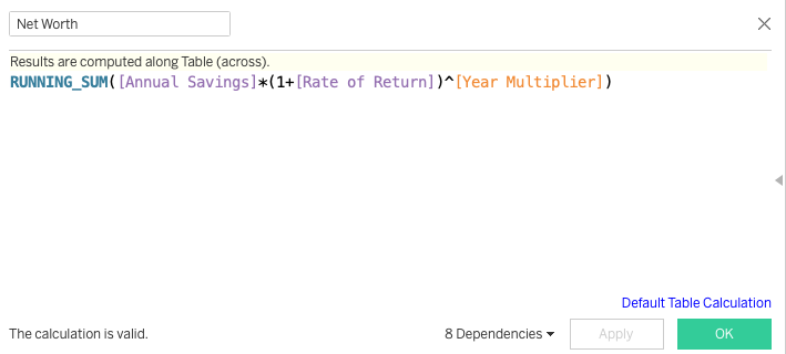
Net worth Gains

Before we get to Net worth Gains, we have to define what our Net Worth is. This will be a running sum of our Annual Savings (the input provided by the user), multiplied by the Rate of Return of investments (defaulted to 7%).

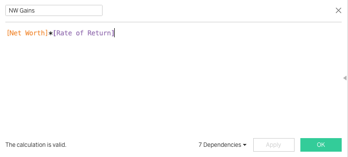
For our Networth Gains calculation, this will be our principal starting balance of Net Worth of the current year, multiplied by the Rate of Return of investments. In our case, we defaulted the Rate of Return to 7%.

With that being said, our “NW Gains” and “Annual Adjusted Income” as dual-axis measures, in aggregation, across number of years, as dimensions, enable us to achieve a converging visualization depicting the year in which our investment returns will begin to exceed our earned income.

Hope you enjoyed this small write-up as much as I did building it!